26 Reshaping
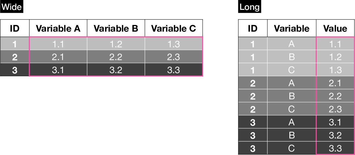
Tabular data can be stored in different formats. Two of the most common ones are wide and long.
A wide dataset contains a single row per case (e.g. patient), while a long dataset can contain multiple rows per case (e.g. for multiple variables or timepoints).
We want to be able to reshape from one form to the other because different programs (e.g. statistical models, plotting functions) expect data in one or the other format for different applications (e.g. longitudinal modeling or grouped visualizations).
R’s reshape() function is very powerful, but can seem intimidating at first, because its documentation is not very clear, especially if you’re not familiar with the jargon.
This chapter includes detailed diagrams and step-by-step instructions to explain how to build calls for long-to-wide and wide-to-long reshaping.
26.1 Long to Wide
26.1.1 Key-value pairs
It is very common to receive data in long format. For example, many tables with electronic health records are stored in long format.
Let’s start with a small synthetic dataset:
dat_long <- data.frame(
    Account_ID = c(8001, 8002, 8003, 8004, 8001, 8002, 8003, 8004,
            8001, 8002, 8003, 8004, 8001, 8002, 8003, 8004),
    Age = c(67.8017038366664, 42.9198507293701, 46.2301756642422,
            39.665983196671, 67.8017038366664, 42.9198507293701,
            46.2301756642422, 39.665983196671, 67.8017038366664,
            42.9198507293701, 46.2301756642422, 39.665983196671,
            67.8017038366664, 42.9198507293701, 46.2301756642422,
            39.665983196671),
    Admission = c("ED", "Planned", "Planned", "ED", "ED", "Planned",
            "Planned", "ED", "ED", "Planned", "Planned", "ED", "ED", "Planned",
            "Planned", "ED"),
    Lab_key = c("RBC", "RBC", "RBC", "RBC", "WBC", "WBC", "WBC", "WBC",
            "Hematocrit", "Hematocrit", "Hematocrit", "Hematocrit",
            "Hemoglobin", "Hemoglobin", "Hemoglobin", "Hemoglobin"),
    Lab_value = c(4.63449321082268, 3.34968550627897, 4.27037213597765,
            4.93897736897793, 8374.22887757195, 7612.37380499927,
            8759.27855519425, 6972.28096216548, 36.272693147236,
            40.5716317809522, 39.9888624177955, 39.8786884058422,
            12.6188444991545, 12.1739747363806, 15.1293426442183,
            14.8885696185238)
)
dat_long <- dat_long[order(dat_long$Account_ID), ]
dat_long
Account_ID Age Admission Lab_key Lab_value
1 8001 67.80170 ED RBC 4.634493
5 8001 67.80170 ED WBC 8374.228878
9 8001 67.80170 ED Hematocrit 36.272693
13 8001 67.80170 ED Hemoglobin 12.618844
2 8002 42.91985 Planned RBC 3.349686
6 8002 42.91985 Planned WBC 7612.373805
10 8002 42.91985 Planned Hematocrit 40.571632
14 8002 42.91985 Planned Hemoglobin 12.173975
3 8003 46.23018 Planned RBC 4.270372
7 8003 46.23018 Planned WBC 8759.278555
11 8003 46.23018 Planned Hematocrit 39.988862
15 8003 46.23018 Planned Hemoglobin 15.129343
4 8004 39.66598 ED RBC 4.938977
8 8004 39.66598 ED WBC 6972.280962
12 8004 39.66598 ED Hematocrit 39.878688
16 8004 39.66598 ED Hemoglobin 14.888570The dataset consists of an Account_ID, denoting a unique patient identifier, Age, Admission, and a pair of Lab_key and a Lab_value columns. The lab data contains information on four lab results: RBC, WBC, Hematocrit, and Hemoglobin.
Use the following figure to understand reshape()’s long-to-wide syntax. You can use it as a reference when building a call to reshape() by following steps 1 through 3.
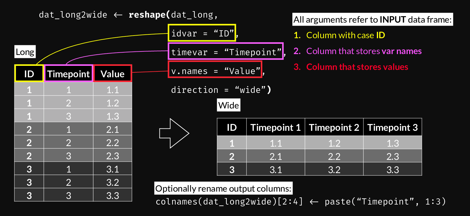
reshape() syntax for Long to Wide transformation.
dat_wide <- reshape(
    dat_long,
    idvar = "Account_ID",
    timevar = "Lab_key",
    v.names = "Lab_value",
    direction = "wide")
dat_wide
Account_ID Age Admission Lab_value.RBC Lab_value.WBC
1 8001 67.80170 ED 4.634493 8374.229
2 8002 42.91985 Planned 3.349686 7612.374
3 8003 46.23018 Planned 4.270372 8759.279
4 8004 39.66598 ED 4.938977 6972.281
Lab_value.Hematocrit Lab_value.Hemoglobin
1 36.27269 12.61884
2 40.57163 12.17397
3 39.98886 15.12934
4 39.87869 14.88857You can optionally clean up column names using gsub(), e.g.
  Account_ID      Age Admission      RBC      WBC Hematocrit Hemoglobin
1       8001 67.80170        ED 4.634493 8374.229   36.27269   12.61884
2       8002 42.91985   Planned 3.349686 7612.374   40.57163   12.17397
3       8003 46.23018   Planned 4.270372 8759.279   39.98886   15.12934
4       8004 39.66598        ED 4.938977 6972.281   39.87869   14.88857
26.1.2 Incomplete data
It is very common that not all cases have entries for all variables. We can simulate this by removing a few lines from the data frame above.
dat_long <- dat_long[-4, ]
dat_long <- dat_long[-6, ]
dat_long <- dat_long[-13, ]
dat_long
Account_ID Age Admission Lab_key Lab_value
1 8001 67.80170 ED RBC 4.634493
5 8001 67.80170 ED WBC 8374.228878
9 8001 67.80170 ED Hematocrit 36.272693
2 8002 42.91985 Planned RBC 3.349686
6 8002 42.91985 Planned WBC 7612.373805
14 8002 42.91985 Planned Hemoglobin 12.173975
3 8003 46.23018 Planned RBC 4.270372
7 8003 46.23018 Planned WBC 8759.278555
11 8003 46.23018 Planned Hematocrit 39.988862
15 8003 46.23018 Planned Hemoglobin 15.129343
4 8004 39.66598 ED RBC 4.938977
8 8004 39.66598 ED WBC 6972.280962
16 8004 39.66598 ED Hemoglobin 14.888570In such cases, long to wide conversion will include NA values where no data is available:
dat_wide <- reshape(dat_long,
    idvar = "Account_ID",
    timevar = "Lab_key",
    v.names = "Lab_value",
    direction = "wide"
)
dat_wide
Account_ID Age Admission Lab_value.RBC Lab_value.WBC
1 8001 67.80170 ED 4.634493 8374.229
2 8002 42.91985 Planned 3.349686 7612.374
3 8003 46.23018 Planned 4.270372 8759.279
4 8004 39.66598 ED 4.938977 6972.281
Lab_value.Hematocrit Lab_value.Hemoglobin
1 36.27269 NA
2 NA 12.17397
3 39.98886 15.12934
4 NA 14.8885726.1.3 Longitudinal data
dat2 <- data.frame(
    pat_enc_csn_id = rep(c(14568:14571), each = 5),
    result_date = rep(c(
        seq(as.Date("2019-08-01"),
            as.Date("2019-08-05"),
            length.out = 5
        )), 4
    ),
    order_description = rep("WBC", 20),
    result_component_value = c(
        rnorm(5, mean = 6800, sd = 3840),
        rnorm(5, mean = 7900, sd = 3100),
        rnorm(5, mean = 8100, sd = 4030),
        rnorm(5, mean = 3200, sd = 1100)
    ))

dat2
pat_enc_csn_id result_date order_description result_component_value
1 14568 2019-08-01 WBC 6794.1975
2 14568 2019-08-02 WBC 7793.9279
3 14568 2019-08-03 WBC 7422.9086
4 14568 2019-08-04 WBC 590.0831
5 14568 2019-08-05 WBC 7638.0087
6 14569 2019-08-01 WBC 12484.3217
7 14569 2019-08-02 WBC 9397.4188
8 14569 2019-08-03 WBC 3704.2248
9 14569 2019-08-04 WBC 5870.5167
10 14569 2019-08-05 WBC 13405.1531
11 14570 2019-08-01 WBC 10212.3834
12 14570 2019-08-02 WBC 9017.2128
13 14570 2019-08-03 WBC 8553.0826
14 14570 2019-08-04 WBC 6002.5413
15 14570 2019-08-05 WBC 2741.2143
16 14571 2019-08-01 WBC 3605.9801
17 14571 2019-08-02 WBC 495.4459
18 14571 2019-08-03 WBC 2861.1247
19 14571 2019-08-04 WBC 5705.4209
20 14571 2019-08-05 WBC 1989.3756In this example, we have four unique patient IDs, with five measurements taken on different days.
Following the same recipe as above, we convert to wide format:
dat2_wide <- reshape(dat2,
    idvar = "pat_enc_csn_id",
    timevar = "result_date",
    v.names = "result_component_value",
    direction = "wide"
)
dat2_wide
pat_enc_csn_id order_description result_component_value.2019-08-01
1 14568 WBC 6794.197
6 14569 WBC 12484.322
11 14570 WBC 10212.383
16 14571 WBC 3605.980
result_component_value.2019-08-02 result_component_value.2019-08-03
1 7793.9279 7422.909
6 9397.4188 3704.225
11 9017.2128 8553.083
16 495.4459 2861.125
result_component_value.2019-08-04 result_component_value.2019-08-05
1 590.0831 7638.009
6 5870.5167 13405.153
11 6002.5413 2741.214
16 5705.4209 1989.37626.2 Wide to Long
Use the following figure to understand reshape()’s wide-to-long syntax. Use it as a reference when building a call to reshape() by following steps 1 through 5. It’s important to note which arguments refer to the input vs. the output data frames.
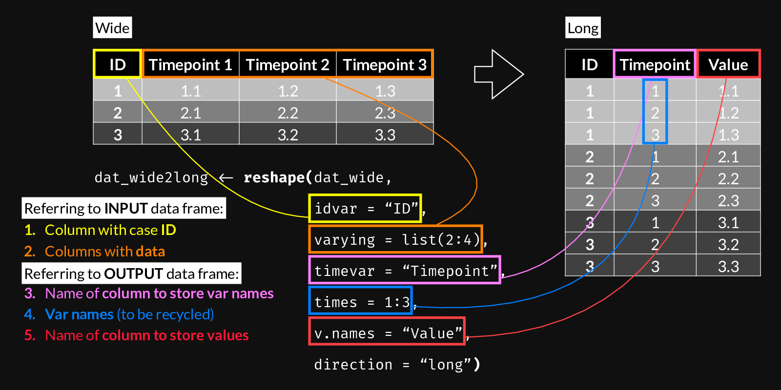
reshape() syntax for Wide to Long transformation.
26.2.1 Example 1: Timepoints
df_wide <- data.frame(
        ID = 1:4,
        Timepoint_A = 11:14,
        Timepoint_B = 21:24,
        Timepoint_C = 51:54)
df_wide
ID Timepoint_A Timepoint_B Timepoint_C
1 1 11 21 51
2 2 12 22 52
3 3 13 23 53
4 4 14 24 54 ID Timepoint Score
1.Timepoint_A 1 Timepoint_A 11
2.Timepoint_A 2 Timepoint_A 12
3.Timepoint_A 3 Timepoint_A 13
4.Timepoint_A 4 Timepoint_A 14
1.Timepoint_B 1 Timepoint_B 21
2.Timepoint_B 2 Timepoint_B 22
3.Timepoint_B 3 Timepoint_B 23
4.Timepoint_B 4 Timepoint_B 24
1.Timepoint_C 1 Timepoint_C 51
2.Timepoint_C 2 Timepoint_C 52
3.Timepoint_C 3 Timepoint_C 53
4.Timepoint_C 4 Timepoint_C 5426.2.2 Example 2: Key-value pairs
set.seed(2022)
df_wide <- data.frame(
  Account_ID = c(8001, 8002, 8003, 8004),
  Age = rnorm(4, mean = 57, sd = 12),
  RBC = rnorm(4, mean = 4.8, sd = 0.5),
  WBC = rnorm(4, mean = 7250, sd = 1500),
  Hematocrit = rnorm(4, mean = 40.2, sd = 4),
  Hemoglobin = rnorm(4, mean = 13.6, sd = 1.5),
  Admission = sample(c("ED", "Planned"), size = 4, replace = TRUE)
)
df_wide
Account_ID Age RBC WBC Hematocrit Hemoglobin Admission
1 8001 67.80170 4.634493 8374.229 36.27269 12.61884 ED
2 8002 42.91985 3.349686 7612.374 40.57163 12.17397 Planned
3 8003 46.23018 4.270372 8759.279 39.98886 15.12934 Planned
4 8004 39.66598 4.938977 6972.281 39.87869 14.88857 Planneddf_long <- reshape(# Data in wide format
data = df_wide,
# The column name that defines case IDs
idvar = "Account_ID",
# The columns whose values we want to keep
varying = list(3:6),
# The name of the new column which will contain all
# the values from the columns above
v.names = "Lab value",
# The values/names, of length = (N columns in "varying"),
# that will be recycled to indicate which column from the
# wide dataset each row corresponds to
times = c(colnames(dat_wide)[3:6]),
# The name of the new column created to hold the values
# defined by "times"
timevar = "Lab key",
direction = "long")
df_long Account_ID Age Admission Lab key
8001.Admission 8001 67.80170 ED Admission
8002.Admission 8002 42.91985 Planned Admission
8003.Admission 8003 46.23018 Planned Admission
8004.Admission 8004 39.66598 Planned Admission
8001.Lab_value.RBC 8001 67.80170 ED Lab_value.RBC
8002.Lab_value.RBC 8002 42.91985 Planned Lab_value.RBC
8003.Lab_value.RBC 8003 46.23018 Planned Lab_value.RBC
8004.Lab_value.RBC 8004 39.66598 Planned Lab_value.RBC
8001.Lab_value.WBC 8001 67.80170 ED Lab_value.WBC
8002.Lab_value.WBC 8002 42.91985 Planned Lab_value.WBC
8003.Lab_value.WBC 8003 46.23018 Planned Lab_value.WBC
8004.Lab_value.WBC 8004 39.66598 Planned Lab_value.WBC
8001.Lab_value.Hematocrit 8001 67.80170 ED Lab_value.Hematocrit
8002.Lab_value.Hematocrit 8002 42.91985 Planned Lab_value.Hematocrit
8003.Lab_value.Hematocrit 8003 46.23018 Planned Lab_value.Hematocrit
8004.Lab_value.Hematocrit 8004 39.66598 Planned Lab_value.Hematocrit
Lab value
8001.Admission 4.634493
8002.Admission 3.349686
8003.Admission 4.270372
8004.Admission 4.938977
8001.Lab_value.RBC 8374.228878
8002.Lab_value.RBC 7612.373805
8003.Lab_value.RBC 8759.278555
8004.Lab_value.RBC 6972.280962
8001.Lab_value.WBC 36.272693
8002.Lab_value.WBC 40.571632
8003.Lab_value.WBC 39.988862
8004.Lab_value.WBC 39.878688
8001.Lab_value.Hematocrit 12.618844
8002.Lab_value.Hematocrit 12.173975
8003.Lab_value.Hematocrit 15.129343
8004.Lab_value.Hematocrit 14.888570or using column names:
                Account_ID      Age Admission    Lab key   Lab value
8001.RBC              8001 67.80170        ED        RBC    4.634493
8002.RBC              8002 42.91985   Planned        RBC    3.349686
8003.RBC              8003 46.23018   Planned        RBC    4.270372
8004.RBC              8004 39.66598   Planned        RBC    4.938977
8001.WBC              8001 67.80170        ED        WBC 8374.228878
8002.WBC              8002 42.91985   Planned        WBC 7612.373805
8003.WBC              8003 46.23018   Planned        WBC 8759.278555
8004.WBC              8004 39.66598   Planned        WBC 6972.280962
8001.Hematocrit       8001 67.80170        ED Hematocrit   36.272693
8002.Hematocrit       8002 42.91985   Planned Hematocrit   40.571632
8003.Hematocrit       8003 46.23018   Planned Hematocrit   39.988862
8004.Hematocrit       8004 39.66598   Planned Hematocrit   39.878688
8001.Hemoglobin       8001 67.80170        ED Hemoglobin   12.618844
8002.Hemoglobin       8002 42.91985   Planned Hemoglobin   12.173975
8003.Hemoglobin       8003 46.23018   Planned Hemoglobin   15.129343
8004.Hemoglobin       8004 39.66598   Planned Hemoglobin   14.888570
Explore the resulting data frame’s attributes:
attributes(df_long)$row.names
[1] "8001.RBC" "8002.RBC" "8003.RBC" "8004.RBC"
[5] "8001.WBC" "8002.WBC" "8003.WBC" "8004.WBC"
[9] "8001.Hematocrit" "8002.Hematocrit" "8003.Hematocrit" "8004.Hematocrit"
[13] "8001.Hemoglobin" "8002.Hemoglobin" "8003.Hemoglobin" "8004.Hemoglobin"
$names
[1] "Account_ID" "Age" "Admission" "Lab key" "Lab value"
$class
[1] "data.frame"
$reshapeLong
$reshapeLong$varying
$reshapeLong$varying[[1]]
[1] "RBC" "WBC" "Hematocrit" "Hemoglobin"
$reshapeLong$v.names
[1] "Lab value"
$reshapeLong$idvar
[1] "Account_ID"
$reshapeLong$timevar
[1] "Lab key"These attributes are present if and only if a long data.frame was created from a wide data.frame as above. In this case, reshaping back to wide format is as easy as calling reshape() on the previously converted data.frame with no arguments:
df_wideagain <- reshape(df_long)
df_wideagain
Account_ID Age Admission RBC WBC Hematocrit Hemoglobin
8001.RBC 8001 67.80170 ED 4.634493 8374.229 36.27269 12.61884
8002.RBC 8002 42.91985 Planned 3.349686 7612.374 40.57163 12.17397
8003.RBC 8003 46.23018 Planned 4.270372 8759.279 39.98886 15.12934
8004.RBC 8004 39.66598 Planned 4.938977 6972.281 39.87869 14.88857Note that the reverse does not work, you need to specify the wide to long reshaping normally.