53  Common Statistical Tests

R includes a large number of functions to perform statistical hypothesis testing in the built-in stats package. This chapter includes a brief overview of the syntax for some common tests along with code to produce relevant plots of your data.

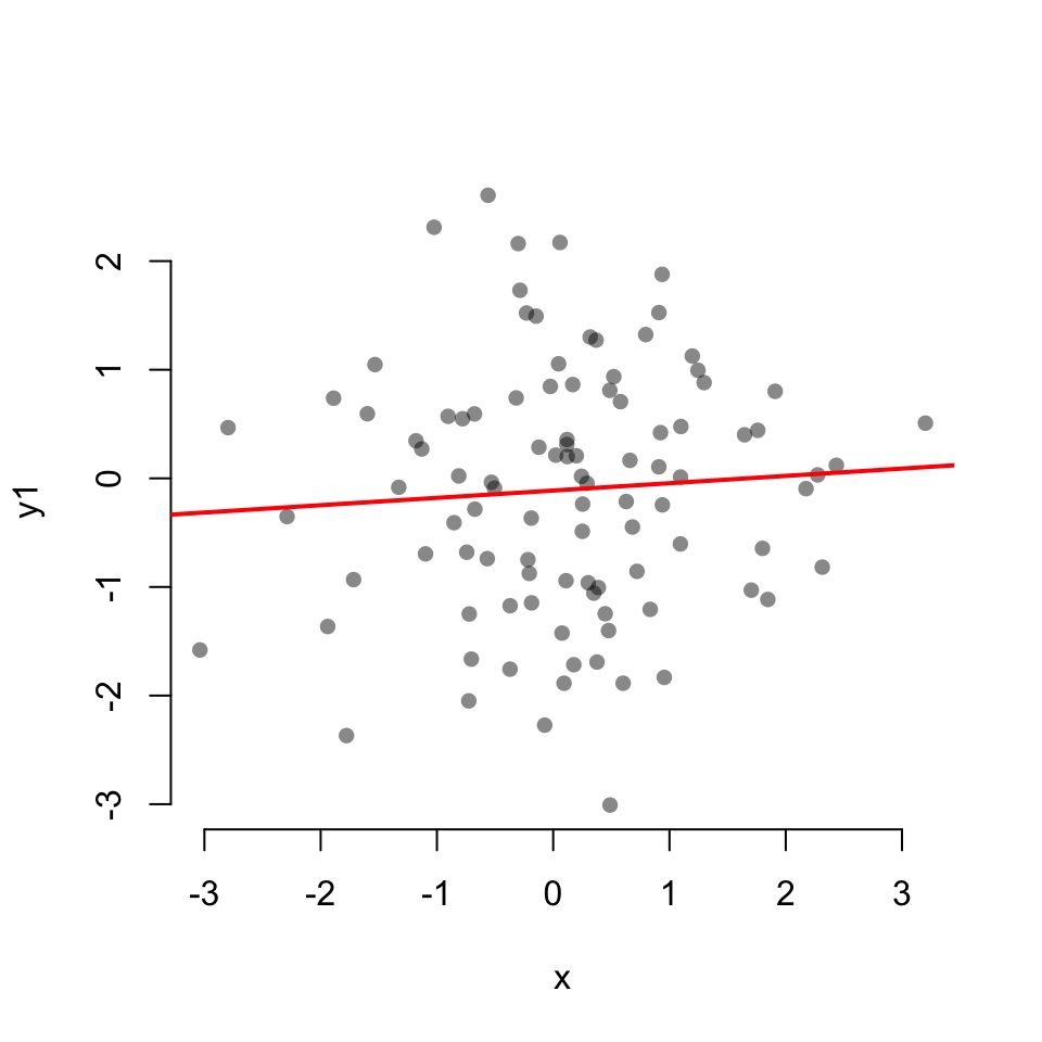
53.1 Correlation test

set.seed(2020)
x <- rnorm(100)
y1 <- 0.1 * x + rnorm(100)
y2 <- 0.3 * x + rnorm(100)
y3 <- x + rnorm(100)/5
y4 <- x^2 + rnorm(100)

Scatterplot with linear fit:

plot(x, y1,
     col = "#00000077",
     pch = 16, bty = "none")
abline(lm(y1 ~ x), col = "red", lwd = 2)

plot(x, y2,
     col = "#00000077",
     pch = 16, bty = "none")
abline(lm(y3 ~ x), col = "red", lwd = 2)

plot(x, y3,
     col = "#00000077",
     pch = 16, bty = "none")
abline(lm(y3 ~ x), col = "red", lwd = 2)

Scatterplot with a LOESS fit

scatter.smooth(x, y4,
               col = "#00000077",
               pch = 16, bty = "none",
               lpars = list(col = "red", lwd = 2))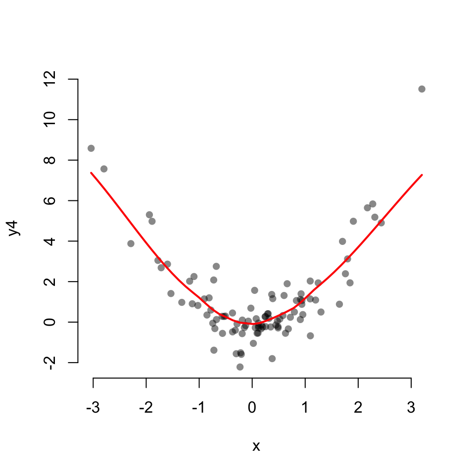

cor.test(x, y1)

    Pearson's product-moment correlation

data:  x and y1
t = 0.66018, df = 98, p-value = 0.5107
alternative hypothesis: true correlation is not equal to 0
95 percent confidence interval:
 -0.1315978  0.2595659
sample estimates:
       cor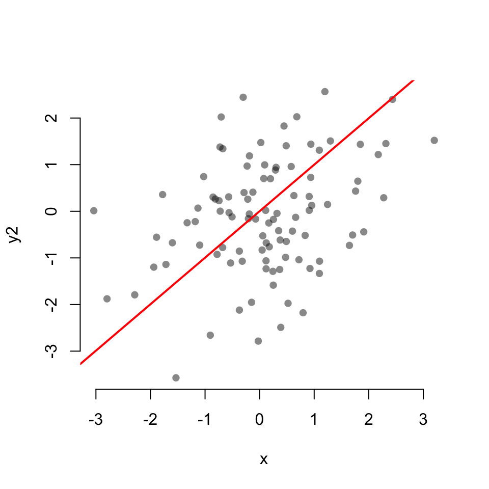 
0.06654026 

cor.test(x, y2)

    Pearson's product-moment correlation

data:  x and y2
t = 3.3854, df = 98, p-value = 0.001024
alternative hypothesis: true correlation is not equal to 0
95 percent confidence interval:
 0.1357938 0.4889247
sample estimates:
      cor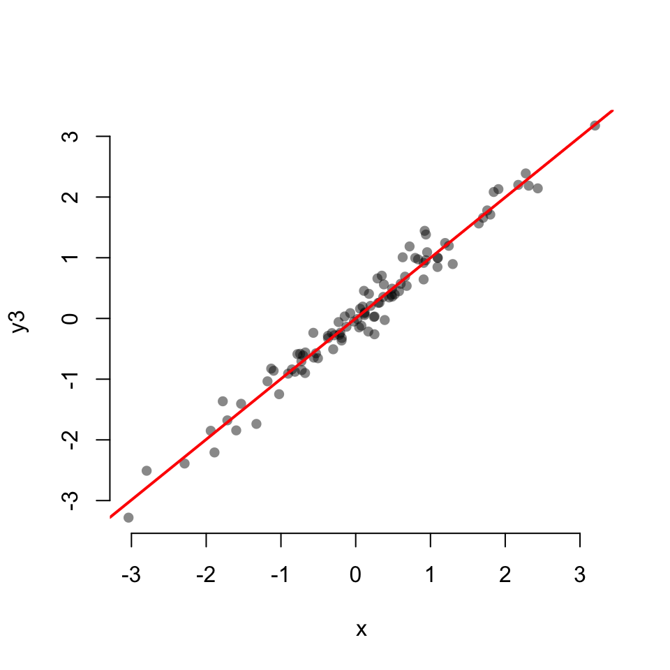 
0.3235813 

cor.test(x, y3)

    Pearson's product-moment correlation

data:  x and y3
t = 53.689, df = 98, p-value < 2.2e-16
alternative hypothesis: true correlation is not equal to 0
95 percent confidence interval:
 0.9754180 0.9888352
sample estimates:
      cor 
0.9834225 

cor.test(x, y4)

    Pearson's product-moment correlation

data:  x and y4
t = 0.66339, df = 98, p-value = 0.5086
alternative hypothesis: true correlation is not equal to 0
95 percent confidence interval:
 -0.1312793  0.2598681
sample estimates:
       cor 
0.06686289 

53.2 Student’s t-test

set.seed(2021)
x0 <- rnorm(500)
x1 <- rnorm(500, mean = 0.7)

For all tests of differences in means, a boxplot is a good way to visualize. It accepts individual vectors, list or data.frame of vectors, or a formula to split a vector into groups by a factor.

boxplot(x0, x1,
        col = "#05204999", border = "#052049",
        boxwex = 0.3, names = c("x0", "x1"))

53.2.1 One sample t-test

t.test(x0)

    One Sample t-test

data:  x0
t = 0.093509, df = 499, p-value = 0.9255
alternative hypothesis: true mean is not equal to 0
95 percent confidence interval:
 -0.08596896  0.09456106
sample estimates:
  mean of x 
0.004296046 

t.test(x1)

    One Sample t-test

data:  x1
t = 15.935, df = 499, p-value < 2.2e-16
alternative hypothesis: true mean is not equal to 0
95 percent confidence interval:
 0.6322846 0.8101311
sample estimates:
mean of x 
0.7212079 

boxplot(extra ~ group, data = sleep,
        col = "#05204999", border = "#052049",
        boxwex = 0.3)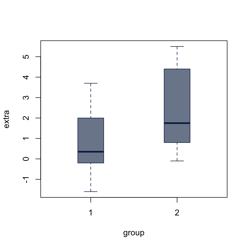

53.2.2 Two-sample T-test

Both t.test() and wilcox.test() (below) either accept input as two vectors, t.test(x, y) or a formula of the form t.test(x ~ group). The paired argument allows us to define a paired test. Since the sleep dataset includes measurements on the same cases in two conditions, we set paired = TRUE.

t.test(extra ~ group, data = sleep, paired = TRUE)

    Paired t-test

data:  extra by group
t = -4.0621, df = 9, p-value = 0.002833
alternative hypothesis: true mean difference is not equal to 0
95 percent confidence interval:
 -2.4598858 -0.7001142
sample estimates:
mean difference 
          -1.58 

53.3 Wilcoxon test

Data from R Documentation:

## Hollander & Wolfe (1973), 29f.
## Hamilton depression scale factor measurements in 9 patients with
##  mixed anxiety and depression, taken at the first (x) and second
##  (y) visit after initiation of a therapy (administration of a
##  tranquilizer).
x <- c(1.83,  0.50,  1.62,  2.48, 1.68, 1.88, 1.55, 3.06, 1.30)
y <- c(0.878, 0.647, 0.598, 2.05, 1.06, 1.29, 1.06, 3.14, 1.29)
depression <- data.frame(first = x, second = y, change = y - x)

53.3.1 One-sample Wilcoxon

wilcox.test(depression$change)

    Wilcoxon signed rank exact test

data:  depression$change
V = 5, p-value = 0.03906
alternative hypothesis: true location is not equal to 0

53.3.2 Two-sample Wilcoxon rank sum test (unpaired)

a.k.a Mann-Whitney U test a.k.a. Mann–Whitney–Wilcoxon (MWW) a.k.a. Wilcoxon–Mann–Whitney test

x1 <- rnorm(500, mean = 3, sd = 1.5)
x2 <- rnorm(500, mean = 5, sd = 2)
wilcox.test(x1, x2)

    Wilcoxon rank sum test with continuity correction

data:  x1 and x2
W = 47594, p-value < 2.2e-16
alternative hypothesis: true location shift is not equal to 0

53.3.3 Two-sample Wilcoxon signed-rank test (paired)

wilcox.test(x, y, paired = TRUE)

    Wilcoxon signed rank exact test

data:  x and y
V = 40, p-value = 0.03906
alternative hypothesis: true location shift is not equal to 0

wilcox.test(x, y, paired = TRUE, alternative = "greater")

    Wilcoxon signed rank exact test

data:  x and y
V = 40, p-value = 0.01953
alternative hypothesis: true location shift is greater than 0

53.4 Analysis of Variance

set.seed(20)
BP_drug <- data.frame(
  Group = factor(rep(c("Placebo", "Drug_A", "Drug_B"), each = 20),
                 levels = c("Placebo", "Drug_A", "Drug_B")),
    SBP = c(rnorm(20, mean = 140, sd = 2.2), rnorm(20, mean = 132, sd = 2.1),
            rnorm(20, mean = 138, sd = 2))
)

boxplot(SBP ~ Group, data = BP_drug,
        col = "#05204999", border = "#052049",
        boxwex = 0.3)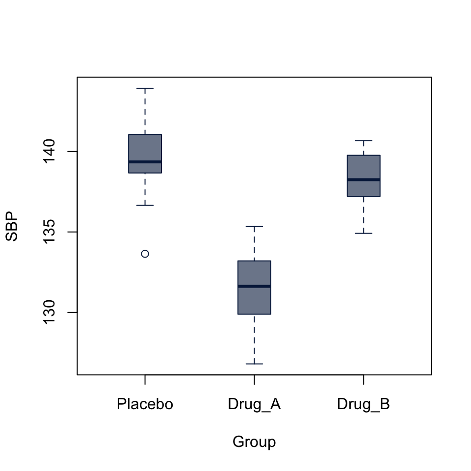

SBP_aov <- aov(SBP ~ Group, data = BP_drug)
SBP_aov

Call:
   aov(formula = SBP ~ Group, data = BP_drug)

Terms:
                   Group Residuals
Sum of Squares  728.2841  264.4843
Deg. of Freedom        2        57

Residual standard error: 2.154084
Estimated effects may be unbalanced

summary(SBP_aov)

            Df Sum Sq Mean Sq F value Pr(>F)    
Group        2  728.3   364.1   78.48 <2e-16 ***
Residuals   57  264.5     4.6                   
---
Signif. codes:  0 '***' 0.001 '**' 0.01 '*' 0.05 '.' 0.1 ' ' 1

The analysis of variance p-value is highly significant, but doesn’t tell us which levels of the Group factor are significantly different from each other. The boxplot already gives us a pretty good idea, but we can follow up with a pairwise t-test

53.4.1 Pot-hoc pairwise t-tests

pairwise.t.test(BP_drug$SBP, BP_drug$Group,
                p.adj = "holm")

    Pairwise comparisons using t tests with pooled SD 

data:  BP_drug$SBP and BP_drug$Group 

       Placebo Drug_A 
Drug_A 2.9e-16 -      
Drug_B 0.065   1.7e-13

P value adjustment method: holm 

The pairwise tests suggest that the difference between Placebo and Drug_A and between Drug_a and Drug_b are highly significant, while difference between Placebo and Drub_B is not (p = 0.065).

53.5 Kruskal-Wallis test

Kruskal-Wallis rank sum test of the null that the location parameters of the distribution of x are the same in each group (sample). The alternative is that they differ in at least one. It is a generalization of the Wilcoxon test to multiple independent samples.

From the R Documentation:

## Hollander & Wolfe (1973), 116.
## Mucociliary efficiency from the rate of removal of dust in normal
##  subjects, subjects with obstructive airway disease, and subjects
##  with asbestosis.
x <- c(2.9, 3.0, 2.5, 2.6, 3.2) # normal subjects
y <- c(3.8, 2.7, 4.0, 2.4)      # with obstructive airway disease
z <- c(2.8, 3.4, 3.7, 2.2, 2.0) # with asbestosis
kruskal.test(list(x, y, z))

    Kruskal-Wallis rank sum test

data:  list(x, y, z)
Kruskal-Wallis chi-squared = 0.77143, df = 2, p-value = 0.68

boxplot(Ozone ~ Month, data = airquality,
        col = "#05204999", border = "#052049",
        boxwex = 0.3)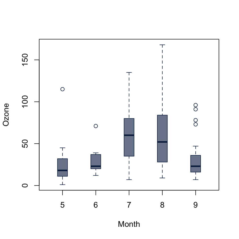

kruskal.test(Ozone ~ Month, data = airquality)

    Kruskal-Wallis rank sum test

data:  Ozone by Month
Kruskal-Wallis chi-squared = 29.267, df = 4, p-value = 6.901e-06

53.6 Chi-squared Test

Pearson’s chi-squared test for count data

Some synthetic data:

set.seed(2021)
set.seed(2021)
Cohort <- factor(sample(c("Control", "Case"), size = 500, replace = TRUE),
                 levels = c("Control", "Case"))
Sex <- factor(
  sapply(seq(Cohort), \(i) sample(c("Male", "Female"), size = 1,
                                  prob = if (Cohort[i] == "Control") c(1, 1) else c(2, 1))))
dat <- data.frame(Cohort, Sex)
head(dat)

   Cohort    Sex
1 Control   Male
2    Case   Male
3    Case   Male
4    Case Female
5 Control Female
6    Case   Male

You can lot count data using a mosaic plot, with either a table or formula input:

mosaicplot(table(Cohort, Sex),
           color = c("orchid", "skyblue"),
           border = NA,
           main = "Cohort x Sex")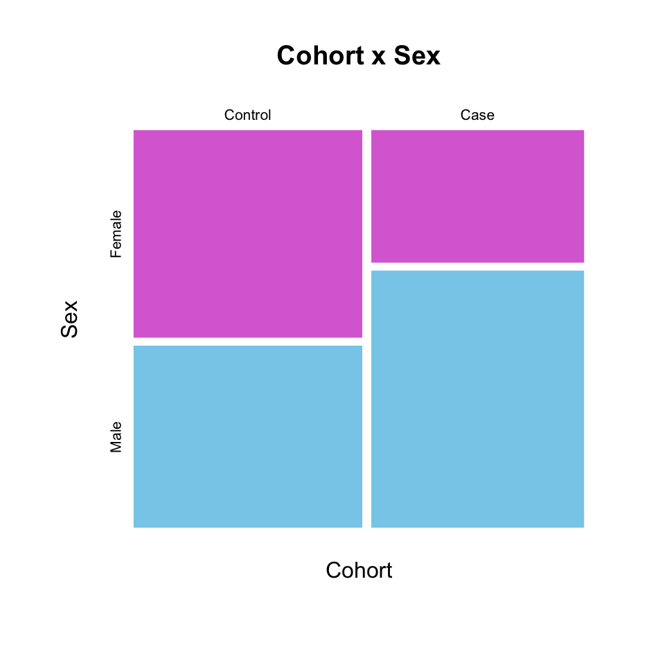

mosaicplot(Cohort ~ Sex, dat,
           color = c("orchid", "skyblue"),
           border = NA,
           main = "Cohort x Sex")

chisq.test() accepts either two factors, or a table:

cohort_sex_chisq <- chisq.test(dat$Cohort, dat$Sex)
cohort_sex_chisq

    Pearson's Chi-squared test with Yates' continuity correction

data:  dat$Cohort and dat$Sex
X-squared = 18.015, df = 1, p-value = 2.192e-05

cohort_sex_chisq <- chisq.test(table(dat$Cohort, dat$Sex))
cohort_sex_chisq

    Pearson's Chi-squared test with Yates' continuity correction

data:  table(dat$Cohort, dat$Sex)
X-squared = 18.015, df = 1, p-value = 2.192e-05

53.7 Fisher’s exact test

Fisher’s exact test for count data

Working on the same data as above, fisher.test() also accepts either two factors or a table as input:

cohort_sex_fisher <- fisher.test(dat$Cohort, dat$Sex)
cohort_sex_fisher

    Fisher's Exact Test for Count Data

data:  dat$Cohort and dat$Sex
p-value = 1.512e-05
alternative hypothesis: true odds ratio is not equal to 1
95 percent confidence interval:
 1.516528 3.227691
sample estimates:
odds ratio 
  2.207866 

cohort_sex_fisher <- fisher.test(table(dat$Cohort, dat$Sex))
cohort_sex_fisher

    Fisher's Exact Test for Count Data

data:  table(dat$Cohort, dat$Sex)
p-value = 1.512e-05
alternative hypothesis: true odds ratio is not equal to 1
95 percent confidence interval:
 1.516528 3.227691
sample estimates:
odds ratio 
  2.207866 

53.8 F Test to compare two variances

x1 <- rnorm(500, sd = 1)
x2 <- rnorm(400, sd = 1.5)
var.test(x1, x2)

    F test to compare two variances

data:  x1 and x2
F = 0.43354, num df = 499, denom df = 399, p-value < 2.2e-16
alternative hypothesis: true ratio of variances is not equal to 1
95 percent confidence interval:
 0.3594600 0.5218539
sample estimates:
ratio of variances 
         0.4335363 

boxplot(x1, x2,
        col = "#05204999", border = "#052049",
        boxwex = 0.3)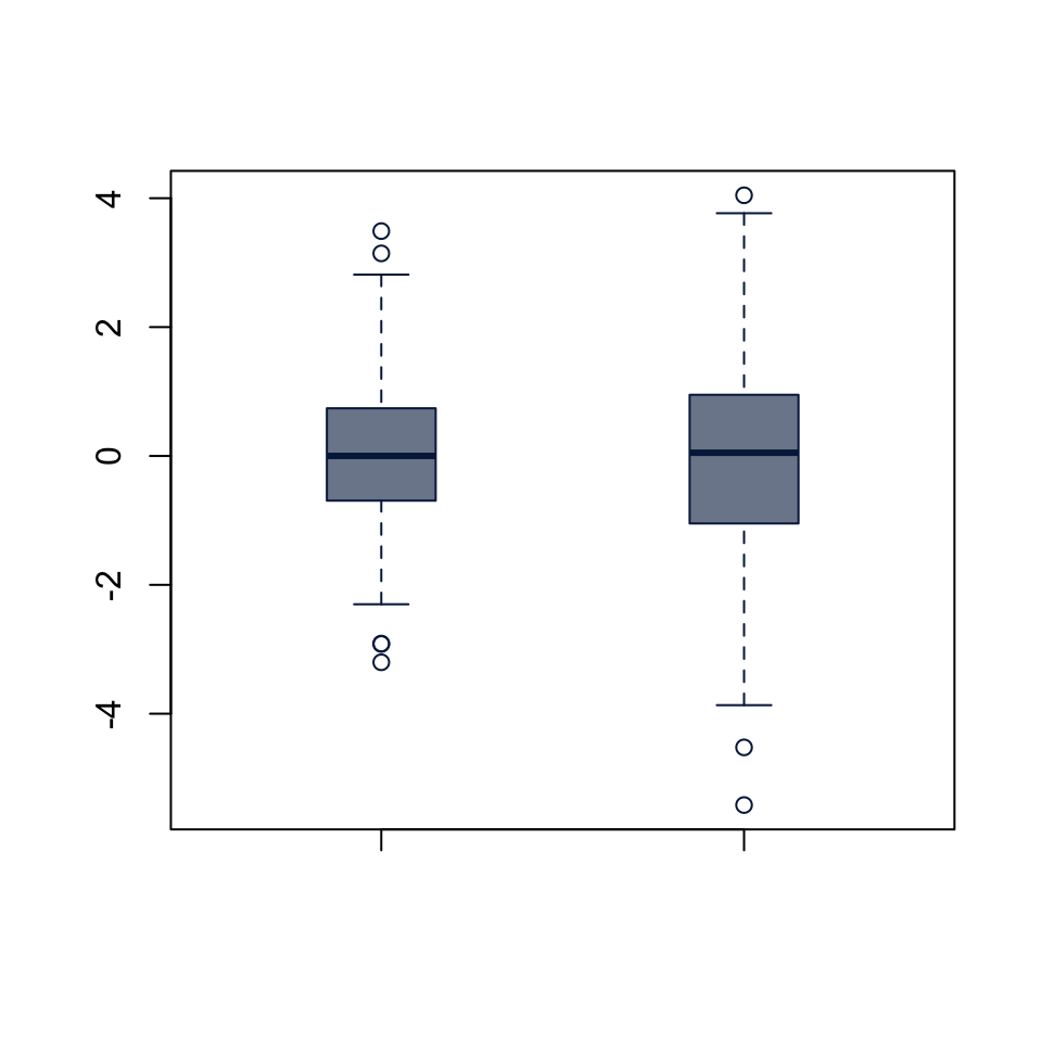

From R Documentation:

x <- rnorm(50, mean = 0, sd = 2)
y <- rnorm(30, mean = 1, sd = 1)
var.test(x, y)                  # Do x and y have the same variance?

    F test to compare two variances

data:  x and y
F = 5.4776, num df = 49, denom df = 29, p-value = 5.817e-06
alternative hypothesis: true ratio of variances is not equal to 1
95 percent confidence interval:
  2.752059 10.305597
sample estimates:
ratio of variances 
          5.477573 

var.test(lm(x ~ 1), lm(y ~ 1))  # same

    F test to compare two variances

data:  lm(x ~ 1) and lm(y ~ 1)
F = 5.4776, num df = 49, denom df = 29, p-value = 5.817e-06
alternative hypothesis: true ratio of variances is not equal to 1
95 percent confidence interval:
  2.752059 10.305597
sample estimates:
ratio of variances 
          5.477573 

53.9 Bartlett test of homogeneity of variances

Performs Bartlett’s test of the null that the variances in each of the groups (samples) are the same.

From the R Documentation:

plot(count ~ spray, data = InsectSprays)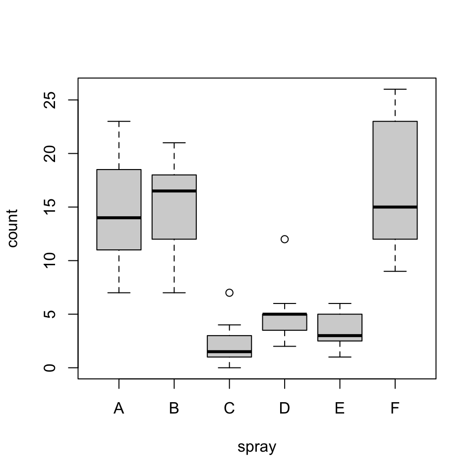

bartlett.test(InsectSprays$count, InsectSprays$spray)

    Bartlett test of homogeneity of variances

data:  InsectSprays$count and InsectSprays$spray
Bartlett's K-squared = 25.96, df = 5, p-value = 9.085e-05

bartlett.test(count ~ spray, data = InsectSprays)

    Bartlett test of homogeneity of variances

data:  count by spray
Bartlett's K-squared = 25.96, df = 5, p-value = 9.085e-05

53.10 Fligner-Killeen test of homogeneity of variances

Performs a Fligner-Killeen (median) test of the null that the variances in each of the groups (samples) are the same.

boxplot(count ~ spray, data = InsectSprays)

# works the same if you do plot(count ~ spray, data = InsectSprays)
fligner.test(InsectSprays$count, InsectSprays$spray)

    Fligner-Killeen test of homogeneity of variances

data:  InsectSprays$count and InsectSprays$spray
Fligner-Killeen:med chi-squared = 14.483, df = 5, p-value = 0.01282

fligner.test(count ~ spray, data = InsectSprays)

    Fligner-Killeen test of homogeneity of variances

data:  count by spray
Fligner-Killeen:med chi-squared = 14.483, df = 5, p-value = 0.01282

53.11 Ansari-Bradley test

Performs the Ansari-Bradley two-sample test for a difference in scale parameters.

ramsay <- c(111, 107, 100, 99, 102, 106, 109, 108, 104, 99,
            101, 96, 97, 102, 107, 113, 116, 113, 110, 98)
jung.parekh <- c(107, 108, 106, 98, 105, 103, 110, 105, 104,
            100, 96, 108, 103, 104, 114, 114, 113, 108, 106, 99)
ansari.test(ramsay, jung.parekh)

Warning in ansari.test.default(ramsay, jung.parekh): cannot compute exact
p-value with ties

    Ansari-Bradley test

data:  ramsay and jung.parekh
AB = 185.5, p-value = 0.1815
alternative hypothesis: true ratio of scales is not equal to 1

x <- rnorm(40, sd = 1.5)
y <- rnorm(40, sd = 2.5)
ansari.test(x, y)

    Ansari-Bradley test

data:  x and y
AB = 963, p-value = 0.005644
alternative hypothesis: true ratio of scales is not equal to 1

53.12 Mood two-sample test of scale

mood.test(x, y)

    Mood two-sample test of scale

data:  x and y
Z = -2.7363, p-value = 0.006213
alternative hypothesis: two.sided

53.13 Kolmogorov-Smirnoff test

Perform a one- or two-sample Kolmogorov-Smirnov test Null: x and y were drawn from the same continuous distribution.

x1 <- rnorm(200, mean = 0, sd = 1)
x2 <- rnorm(200, mean = -0.5, sd = 1.5)
ks.test(x1, x2)

    Asymptotic two-sample Kolmogorov-Smirnov test

data:  x1 and x2
D = 0.35, p-value = 4.579e-11
alternative hypothesis: two-sided

53.14 Shapiro-Wilk test of normality

set.seed(2021)
x <- rnorm(2000)
y1 <- 0.7 * x
y2 <- x + x^3

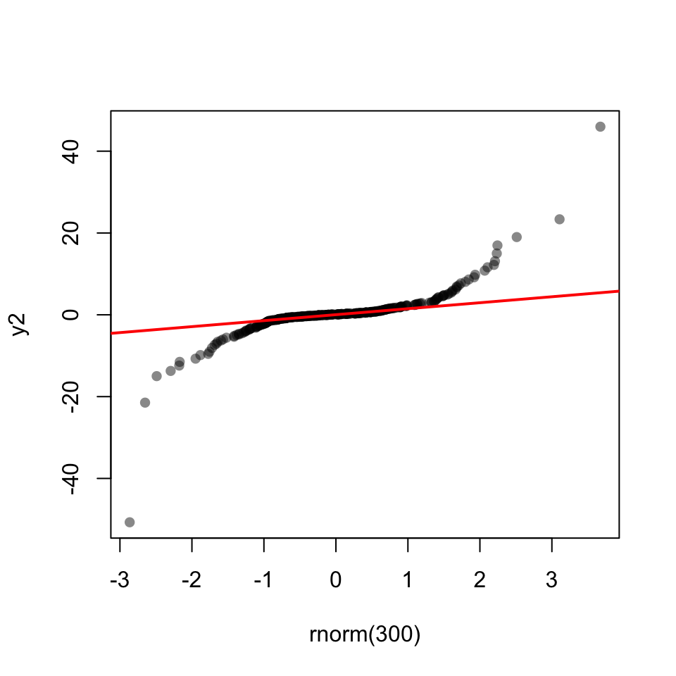
53.14.1 Q-Q Plot

qqplot(rnorm(300), y1, pch = 16, col = "#00000077")
qqline(y1, col = "red", lwd = 2)

qqplot(rnorm(300), y2, pch = 16, col = "#00000077")
qqline(y2, col = "red", lwd = 2)

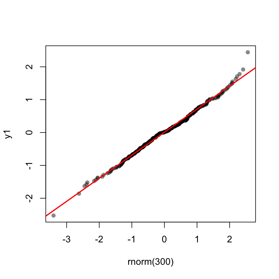
53.15 Shapiro-Wilk test

shapiro.test(y1)

    Shapiro-Wilk normality test

data:  y1
W = 0.99952, p-value = 0.9218

shapiro.test(y2)

    Shapiro-Wilk normality test

data:  y2
W = 0.72936, p-value < 2.2e-16

53.16 Resources

• Regression Methods in Biostatistics: Linear, Logistic, Survival, and Repeated Measures Models